How To Get Minus Value In Excel
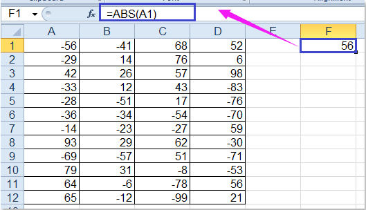
How to remove leading minus sign from numbers in Excel. Suppose you want to subtract 50 from 500.
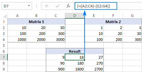
How To Subtract A Number From A Range Of Cells In Excel
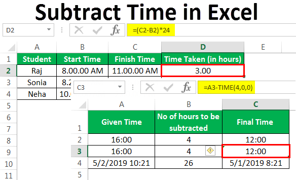
However the time values that on subtraction exceed 24 hours60 minutes60 seconds are ignored by Excel.
How to get minus value in excel. Follow these steps to subtract numbers in different ways. There are two aspects to it one is if you have alphanumeric values in a column and you would like to insert a minus sign before the value so the resultant value is text string only. You have to use the mathematical operator minus sign - to subtract two numbers.
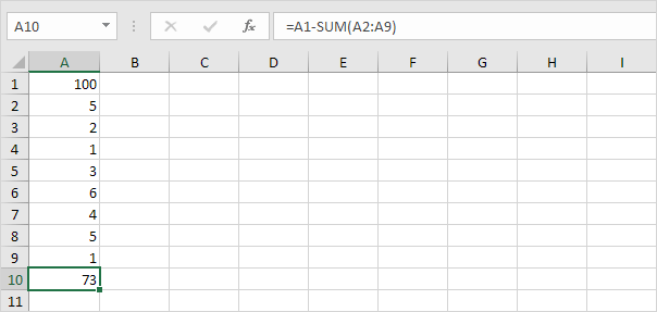
Sum ignore negative values. When you type 10 into Excel Excel sees it as the value 01. Excel does this with all percentage values.
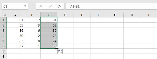
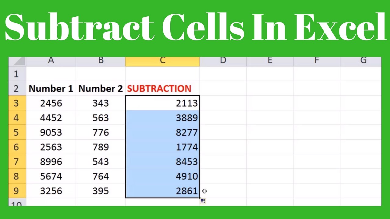
Select all of the rows in the table below then press CTRL-C on your keyboard. Next select cell C1 click on the lower right corner of cell C1 and drag it down to cell C6. Enter this formula into a blank cell where you want to put the result SUMIFA1D90 see screenshot.
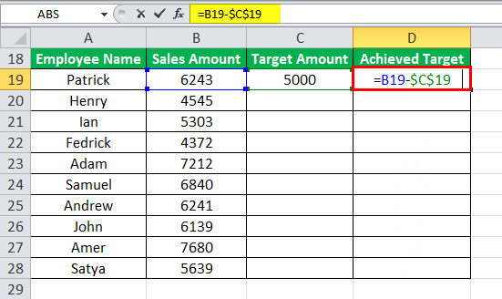
If you want to keep minus before number you can select Custom in Category list then select or enter 0_. In this example cell D6 has the budgeted amount and cell E6 has the actual amount as a negative number. Then press Enter key to get the result see screenshot.
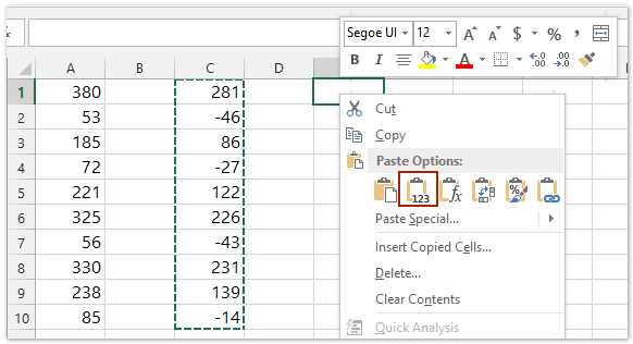
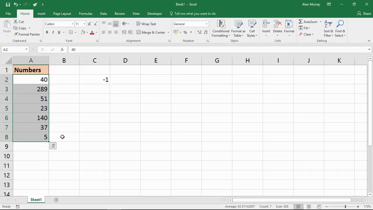
Add -1 to a cell and copy to the clipboard Select the negative numbers you want to convert Use Paste Special. Select the cells which have the negative percentage you want to mark in red. For subtraction of time values less than 24 hours we can easily subtract these by using the - operator.
Average ignore negative values. To switch between viewing the results and viewing the formulas press CTRL grave accent on your. 3And in the Change Sign of Values dialog box select Change all positive values to negative option.
Enter the formula below we will just concatenate a minus sign at the beginning of the value as show below. Type the first number followed by the minus sign followed by the second number. Start by right-clicking a cell or range of selected cells and then clicking the Format Cells command.
To enter the formula in your worksheet do the following. -0 in Type field. Type a positive value in one cell and a negative value in another.
First select a cell to add the formula to. Select the numbers and then right click to shown the context menu and select Format Cells. Right click the selected cells and select Format Cells in the right-clicking menu.
But you get SUM function to add numbers or range of cells. For example input 25-5 in the function bar and press. 2Click Kutools Content Change Sign of Values see screenshot.
In the Format Cells dialog box you need to. F6 has the formula SUM D6E6. If you have installed Kutools for Excel you can change positive numbers to negative as follows.
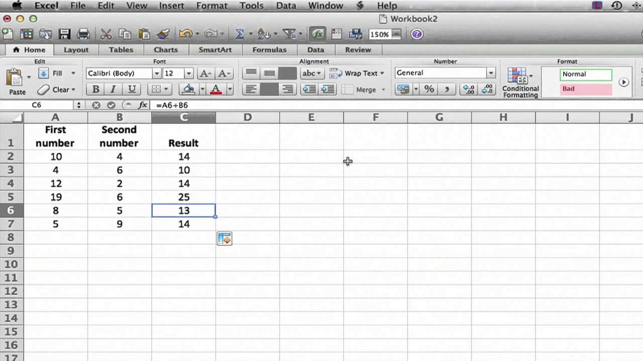
In the Format Cells dialog under Number tab select Number from the Category list and the go to the right section and type 0. 50 is 05 75 is 075 and so on. In a third cell use the SUM function to add the two cells together.
1Select the range you want to change. SUM B2H2-SMALL B2H21 COUNT B2H2-1 into a blank cell where you want to return the result and drag the fill handle down to the cells that you want to apply this formula and all the cells in each row have been averaged ignoring the lowest number see screenshot. It has become quite easy to perform operations like add or subtract different time and date values with Excel.
4Then click OK or ApplyAnd all of the positive numbers have been converted to negative. If you only need to convert negative numbers once you can convert in-place with Paste Special. Then click in the Excel function bar and input followed by the values you need to deduct.
First subtract the value in cell B1 from the value in cell A1. This provides you with the ultimate control over how the data is displayed. Complete the formula by pressing the Enter key.
In Excel you will not find any function called SUBTRACT that will perform the subtraction operation. Create a Custom Negative Number Format You can also create your own number formats in Excel. Mark negative percentage in red by creating a custom format.
In the previous example you were actually asking excel to subtract 01 from 83279 instead of reducing the number by 10. To average ignore the negative values please use this formula. In a cell where you want the result to appear type the equality sign.
Take a look at the screenshot below. In the worksheet select cell A1 and then press CTRLV.
How To Remove Negative Sign From Numbers In Excel
How To Subtract In Excel Easy Excel Formulas
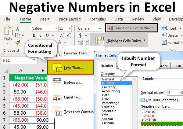
Negative Numbers In Excel Top 3 Ways To Show Negative Number

Subtraction Formula In Excel How To Subtract In Excel Examples
Subtraction Formula In Excel How To Subtract In Excel Examples

How To Change Negative Number To Zero In Excel

How To Change Positive Numbers To Negative In Excel
Excel Tip Make Number Negative Convert Positive Number To Negative Youtube

Excel Formula Change Negative Numbers To Positive Exceljet
How To Subtract Cells In Microsoft Excel 2017 Youtube
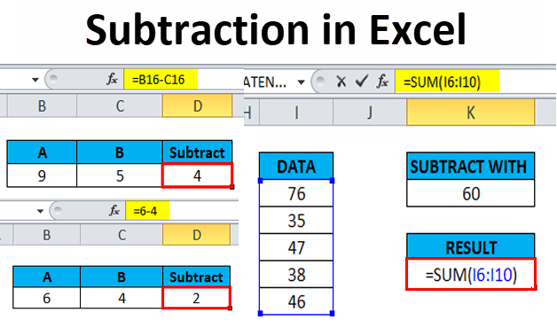
Subtraction In Excel How To Use Subtraction Operator In Excel
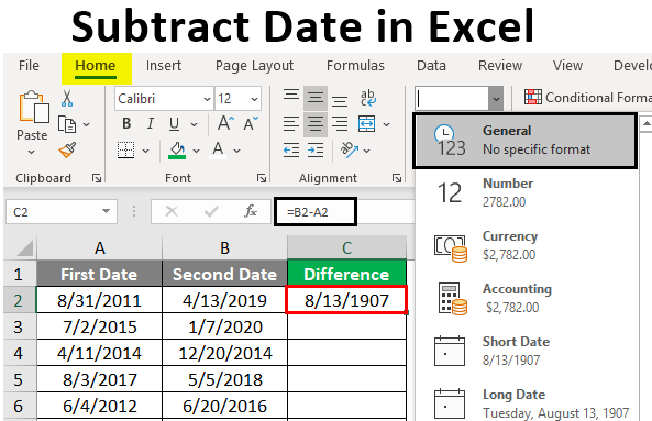
Subtract Date In Excel How To Subtract Date In Excel Examples
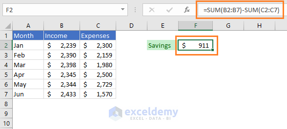
Adding And Subtracting In Excel In One Formula Exceldemy
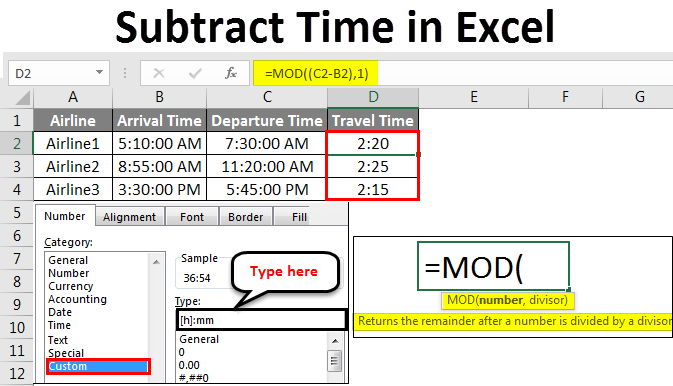
Subtract Time In Excel Excel Formula To Subtract Time Values
How To Subtract In Excel Cells Columns Percentages Dates And Times
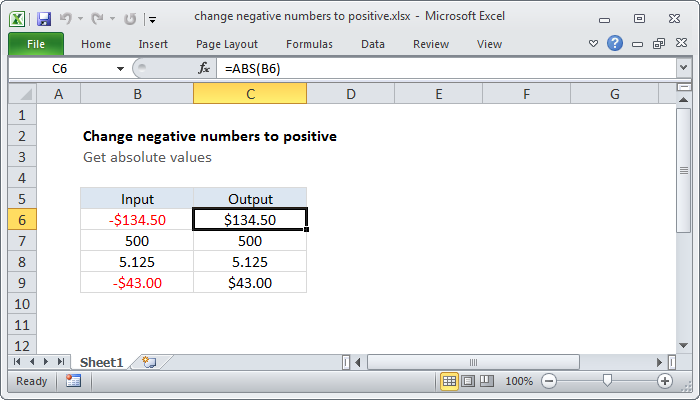
Excel Formula Change Negative Numbers To Positive Exceljet
How To Subtract In Excel Easy Excel Formulas
Subtract Time In Excel How To Subtract Time In Excel Examples
Adding Subtracting Vertical Columns In Excel Ms Excel Tips Youtube